Crosstalk
Engineers spend careers suppressing the signals that leak between neighbouring wires. Two simulated experiments asked whether that leak, or the delay inside a wire, could do a neural network’s job instead.Can a delay line be the neural network?

The player runs both experiments side by side, replaying recorded runs and computing the rest in the browser. The cards below it replay four of the results.
Both architectures, running
Squashed near zero: the summers assume full drive, a matched ladder delivers about half. The article measured accuracy 0.17 as designed and 0.87 with the gain trimmed by 8.98 dB. The plot is the recorded sweep; the board is computed here with the trained layer-1 kernels, first four of eight outputs.
Put two copper traces close together on a circuit board and they start to talk. A pulse sent down one appears, a little later and a little distorted, on the other: a leak called crosstalk. Delay Tensor, the first half of this project, puts the leak to use. It sends a waveform into a bundle of eight coupled lines, records every line at every moment, and hands the recordings to a simple linear classifier. The approach is called reservoir computing: a fixed, untrained system scrambles a signal into a richer form that a simple readout can learn from.
Eight lines side by side, each leaking into the next
Only the readout learns. To see whether the bundle helps, the same readout is also trained on the raw waveform.
The bundle in the drawing has not been built, and the software does not simulate a circuit. Its design notes call it “a physical metaphor, not a circuit solver”: a short NumPy loop that imitates delay, loss, leakage between neighbours and a soft ceiling on amplitude. Sections 7 to 9 test how close that imitation comes to real wires.
The simulation advances in steps of 20 nanoseconds, called slots. A waveform of 64 samples is fed in one sample per slot, and after every slot the state of all eight wires is written down, giving 8 × 64 = 512 numbers per waveform. At each step a wire keeps 99.5% of its previous value, adds the incoming sample scaled by its own fixed gain, adds a share of its two neighbours’ values set by a fixed mask, and passes the total through tanh, a function that squashes large values towards ±1.
A fixed coupling mask: eight wires by 64 slots
What one wire does in one slot
The mask decides how loudly each wire hears its neighbours. In the project’s first version it was drawn so narrowly that every entry came out at 0.5, which made every connection identical and the mask pointless. Redrawn properly, its entries range from 0.02 to 0.955, with a mean of 0.496.
Three reservoir configurations
| Config name | Wires × slots | Nodes | Duration | Neighbour coupling k1 |
|---|---|---|---|---|
| tensor_8x64 | 8 × 64 | 512 | 1,280 ns | 0.08 |
| tensor_16x128 | 16 × 128 | 2,048 | 2,560 ns | 0.06 (0.01 between wires two apart) |
| mnist_8x784 | 8 × 784 | 6,272 | 15,680 ns | 0.08 |
Every test uses the same readout, a standard logistic regression with identical settings and data splits. The only thing that changes is what it reads: the raw samples, or the 512 recorded states.
The first test is a sanity check: telling apart six kinds of short waveform, including sine bursts, square bursts, chirps and pulses, with amplitudes matched so that only shape and timing differ. There are 64 examples of each, and a quarter are held back for testing.
A sine burst and a square burst look almost the same to the reservoir
Six-way classification · tensor_8x64
| Seed | Raw samples | Delay Tensor | Difference |
|---|---|---|---|
| 1234 | 0.833 | 0.844 | +0.010 |
| 1235 | 0.865 | 0.885 | +0.021 |
| 1236 | 0.844 | 0.854 | +0.010 |
| Mean ± sd | 0.847 ± 0.016 | 0.861 ± 0.022 | +0.014 ± 0.006 |
The reservoir does better on every run, but never by more than the runs vary among themselves. Both readouts make only one kind of mistake, confusing sine bursts with square bursts; the other four shapes are identified perfectly. Across three runs the reservoir gets four more of those 96 cases right, 56 against 52, a margin the project’s own report describes as modest.
Temporal XOR is the test a reservoir should pass. Each waveform may carry a pulse early, at sample 16, and another late, at sample 48. The answer is yes when exactly one pulse is present, and no when there are two or none. A linear classifier looking at the raw samples cannot express “one or the other but not both”, because it weighs each sample independently.
Temporal XOR: both pulses, neither, or just one
On raw samples the classifier reaches 0.724 accuracy, mostly by answering yes when the answer is no (45 of 98 such cases across three runs). With the reservoir it gets 191 of 192 right, and reruns in October reproduced the figures exactly.
MNIST, the standard benchmark of 70,000 handwritten digits, was never designed with a reservoir in mind. Each 28 × 28 pixel image is read row by row as a waveform of 784 samples, one per slot, which gives 6,272 numbers per digit. All 60,000 training and 10,000 test images are used in their standard order, so the result can be compared with published ones.
At 2.8 gigabytes, those numbers would crowd the 8 GB laptop that ran the experiment, so they are streamed from disk and the classifier is trained in batches. A small neural network with one hidden layer, trained on the raw pixels, runs alongside as a reference because, as a comment in the code puts it, without one 0.91 and 0.92 are just two numbers.
Delay Tensor against raw samples on three tasks
Eight times as many numbers buy a tenth of a percentage point: 0.9146 accuracy against 0.9136, a difference smaller than its own uncertainty (+0.0011 ± 0.0014), and on one of the three runs the reservoir does worse. The small neural network beats both by 6.4 points. Digit by digit, the reservoir helps slightly with 2s and 6s and costs 2.2 points on 8s.
Where Delay Tensor helps and hurts on each digit
The project’s own report puts the edge inside run-to-run noise. This was the first MNIST run on record and is not yet in the README’s results table.
Why does the reservoir solve XOR? Its design notes credit memory: the coupled wires hold on to the first pulse until the second arrives. If that were true, cutting the coupling or shortening the memory should break it. So each was switched off in turn, and so was the tanh, one change at a time with three runs each.
Switching off coupling, memory and the tanh, one at a time
With the neighbouring wires disconnected, temporal XOR still scores 1.000. With the tanh removed, it scores 0.531.
Coupling turned out not to matter. With the neighbours disconnected, or with coupling anywhere from 0.02 to 0.32, XOR stayed at 1.000. Shortening the memory so far that a value halves every 20 nanoseconds, and nothing of the first pulse survives to the second, also left it at 1.000. Replacing tanh with a straight line dropped it to 0.531 ± 0.196, no better than guessing. Even reading a single wire instead of all eight barely mattered for XOR (0.990), though it cost four points on the six-waveform test (0.816).
The likely explanation is simpler than memory. Because the pulses always arrive at the same two moments, any fixed nonlinear distortion of the signal lets a linear classifier separate two pulses from none, and the tanh applied at every step supplies exactly that. Varying the pulse times would force the reservoir to remember, and would finally test what the coupling is for. That experiment has not been run.
The six-waveform test moved a little with coupling, from 0.858 with none to 0.875 at four times the default, but all the results sit within about two standard deviations of one another. A reservoir twice the size, 16 wires by 128 slots, scored the same as the original on both tasks.
Run for this piece on the project’s code and configs; the numbers are not taken from the project’s results. Each run changes one setting from tensor_8x64; seeds 1234 to 1236; the raw-sample baselines are unchanged at 0.847 and 0.724.
A loop in NumPy is not a circuit, so a separate test bench checks that a circuit simulator, ngspice, produces the same numbers. A circuit has no clock stepping through slots, so the bench lays the slots out in space instead, as a chain of stages. Each term of the update becomes a current fed into a 1-ohm resistor, which turns the summed current into a voltage, and a component that behaves like tanh sits after the sum.
Four waveforms through the 8-wire, 64-slot reservoir become 2,048 stages and 11,953 lines of circuit description, solved in a single pass with tolerances close to the limits of the arithmetic.
ngspice and NumPy agree to the last digit
The two programs agree to the last digit a computer can hold. The largest difference anywhere is 5.27e-16 (ngspice +0.162703485466625, NumPy +0.162703485466624), a single rounding step, and it does not grow along the chain. Writing the bench also turned up a bug in how the circuit version applied tanh.
The bench checks the translation of the equations into a circuit, not any physical hardware. It runs with noise off, so noise and jitter are not covered.
Newer benches model the physical wires the loop stands in for. Three kinds of line, described by their resistance, inductance, capacitance and leakage per unit length, are chopped into short sections, simulated in ngspice, and checked against exact mathematical models and, for the microstrip, against the independent RF library scikit-rf.
Simulated line types
| Line | Conductors | Length | Sections | Defined by |
|---|---|---|---|---|
| 4-line PCB bus | 4 | 100 mm | 64 | electrical matrices: C tridiagonal, L falling off with distance |
| Microstrip pair | 2 | 80 mm | 48 | geometry: 1.5 mm lines, 0.4 mm gap, 0.8 mm FR-4 |
| LC ladder | 2 | 10 mm | 4 | lumped elements: the coarsest case the pipeline has to handle |
Two microstrip lines 0.4 mm apart, in cross-section
Through path and crosstalk, 10 MHz to 3 GHz
From 10 MHz to 3 GHz, ngspice matches the exact model of the sectioned line to within 1e-11 to 1e-13, and the sectioned line comes within about 1% of a continuous one. The tightly coupled microstrip pair is the extreme case (coupling k = 0.755): by about 370 MHz, half the power has gone from the path the signal was sent down, and the far end of the neighbouring line picks up a signal only 3.7 dB weaker than the input. As a reservoir that is a lot of mixing; as a bus it is unusable.
A pulse crosses the coupled pair in 464.8 ps
A 1-volt pulse takes 464.8 picoseconds to cross the 80 mm pair, a little faster than the 481.6 ps predicted, because of the two ways the pair can carry a signal, one travels faster (0.434 ns against 0.535 ns for the other). On the cleaner four-line bus the pulse takes 595 ps against 577.7 ps predicted. Converting the pulse’s journey into frequencies reproduces the frequency sweep to within 0.58% of peak.
For a single line, scikit-rf gives an impedance of 51.12 to 51.17 ohms between 0.1 and 5 GHz, against 51.35 ohms from the textbook formula. Modelling the copper’s 35-micrometre thickness widens the gap from 0.45% to 2%, so thickness accounts for most of it. Loss is 3.64 dB per metre at 1 GHz.
Joining the two halves would mean putting a real line inside the reservoir. A tool for that exists: it fits a compact mathematical model to how a line responds to a pulse, and the reservoir accepts the result as its coupling, provided the model is stable. On made-up test systems it recovers the answer to 1e-12.
No real line has yet been fed through it into a classification task. A quick attempt for this article, on the four-line bus, fitted badly (41% error at order 8, 21% at order 16) and gave models just past the stability limit (spectral radius 1.001 to 1.003), which the reservoir would refuse. The timescales also clash: the lines respond in hundreds of picoseconds, while the reservoir’s clock ticks every 20 nanoseconds, about forty times slower.
Until an extracted line runs as the reservoir, every accuracy figure before section 10 describes the recurrence from section 2, not a physical line.
Delay lines were among the first computer memories. The EDVAC report of 1945 described them, and the EDSAC computer kept its data in 32 tubes of mercury, each holding 560 bits as pulses of sound travelling from one end to the other, where they were caught and sent round again. A tap partway along such a line reads the signal as it was a fixed time ago. Weighted taps added together make a filter (Kallmann, 1940); learnable weights and a squashing function make one layer of a time-delay neural network (Waibel, 1989).
Crosstalk, the second half of the project, builds that layer with as little hardware as possible. Each weight can take only three values: a tap wired to the circuit that adds signals counts as +1, a tap wired to the one that subtracts them counts as −1, and an unconnected tap counts as 0. That makes it a ternary network, the restriction used by Microsoft’s BitNet b1.58 language models, and the weights need no memory, because they are the wiring. Each layer is a grid of resistor pads, two for every pairing of tap and output, and training decides which pads receive a resistor.
As a result, the file that tells an assembly machine where to place parts is the trained network. The design uses three boards, called tiles, each with eight delay lines and eight outputs; their placement files list 85, 315 and 316 resistors, and a script checks that these match the trained weights exactly. Each output takes the difference of its two sums and feeds a matched pair of transistors, whose response is itself a tanh, with a width set by physics: , about 51.7 mV at room temperature. A track-and-hold circuit then hands the result to the next tile in step with the clock.
Trained networks are usually pictured as grids of shaded squares, one per weight. Here each weight is a resistor that is either present or absent, so the same picture becomes a map of solder pads.
Weights of a CNN and of the Crosstalk network, side by side
Training rounds each weight to −1, 0 or +1 on the way forward and lets the gradient pass straight through the rounding on the way back. A microcontroller handles the final steps (pooling, the eight-way readout and the decision), while the delays, the weighted sums and the nonlinearity stay analogue. None of these ideas is new. Pour and Ha (ISCAS 2025) ran an RF recurrent network on a tapped transmission line, Woo, Jung and Mukhopadhyay (2024) built ternary modulation recognition on an FPGA, and Tank and Hopfield used analogue delays in 1987. What the project adds is the whole chain: one set of trained weights carried through four levels of simulation to a routed circuit board, with every gap reported.
The task is recognising how a radio signal is modulated, choosing among eight schemes (OOK, BPSK, QPSK, 8PSK, 16QAM, 2FSK, 4FSK and GMSK) from snippets of 128 samples. The signals are synthetic, 16,000 for training and 4,000 for testing, at signal-to-noise ratios from 0 to 20 dB with random carrier phase. The results rank the project’s models against one another and cannot be compared with published RadioML scores.
Accuracy of nine models on one modulation task
On accuracy, the delay-line network trails the conventional options. A conventional neural network of the same shape, run in floating point, scores 0.909 against its 0.806, and a classical method built on signal statistics (cumulants), with just 208 parameters and no gradient-descent training, scores 0.875. Giving the delay-line network a floating-point final layer, which costs nothing since that layer runs on the microcontroller anyway, recovers part of the gap (0.851). Small fully connected networks fed raw samples cannot cope with the random phase and stall at 0.261 and 0.542; given phase-independent features, one with 992 parameters reaches 0.783.
Cost of one classification · estimates
| Quantity | Crosstalk | 1-D CNN |
|---|---|---|
| Adds | 93,376 | 151,616 |
| Multiplies | 3,144 | 147,528 |
| tanh evaluations | 3,072 | 3,072 |
| Arithmetic energy, 45 nm datapath | ≈ 209 nJ | ≈ 796 nJ |
| Board, 216 mA at 5 V for ≈ 150 µs | ≈ 162 µJ | — |
| STM32G474 running the CNN, lower bound | — | ≥ 84 µJ |
Counting only arithmetic, the delay-line network needs about a quarter of the energy. Built as a board full of op-amps, it would use about 774 times that estimate, up to about twice the minimum for a microcontroller running the more accurate network. At this size the analogue board wins on neither accuracy nor energy. Its one advantage is that the weights cost nothing to store.
The first plan for a physical delay line used coaxial cable, and it could not be built. Each tap needed up to 1.12 microseconds of RG-58 cable, eight lines per layer, losing an estimated 32 dB per microsecond with nothing to boost the signal along the way. One piece of that work survived: a bit-exact simulation of the arithmetic (the E tier in section 13) matched a Verilog hardware description across 202,752 values without a single mismatch.
Its replacement is a ladder of ordinary surface-mount inductors and capacitors, 56 sections of 120 µH and 120 pF, so , 120 ns per section, an ideal cut-off of 2.65 MHz, and a tap every 8 sections. How much signal survives then depends on the inductors’ quality factor, Q. Reaching the last tap at the highest usable frequency costs about 9.6 dB at Q = 10 and about 3.2 dB at Q = 30.
Loss at each of eight taps along one LC line
No inductor on the market met the wish list: 120 µH, shielded, self-resonant above 5 MHz and under 8 ohms. The part chosen is unshielded, with 3.3 ohms of resistance, self-resonance at 3.3 MHz and a guaranteed Q of only 10; the typical Q of 30 is an assumption, because the datasheet gives only the minimum. Symbols arrive at 125,000 a second, eight samples each, and at 250 kHz the simulated loss between first and last tap is 2.26 dB even at the minimum Q. The first job for anyone building it is measuring Q on twenty real parts.
Simulation tiers
| Tier | What is simulated | Not modelled | Result for the board-trained network |
|---|---|---|---|
| V · virtual | ideal-arithmetic NumPy, with the FIR filter response of the ngspice-simulated ladder as the “board line” reference | every physical effect except the line response | 0.878 board line · 0.655 ideal line |
| E · emulated | 8-bit fixed point, bit-for-bit against Verilog RTL | all analog effects | earlier phase-1 networks only, not the board-trained one: 198,144 values, 0 mismatches |
| C · circuit | ngspice on the KiCad-exported tile netlist, two fixes applied | layout, crosstalk, noise | 0.8505 at Q 10 · 0.8588 at Q 30 (calibrated model) |
| P · parasitics | scikit-rf cascade of ABCD matrices with parasitics and mutual inductance; Monte Carlo over 1,000 simulated boards | electromagnetic field effects and layout | 0.8705 at Q 10 · 0.872 at Q 30 |
A ladder of real components is an imperfect delay: it rings, it loses signal, and its delay varies with frequency. So the network is trained on the line it will actually sit on. A single pulse sent through the simulated ladder and sampled at each tap gives a short filter for every tap, and every training pass mixes the responses for Q = 10 and Q = 30 and shifts each tap’s timing by up to 14% of a symbol. Through this realistic line, the network trained on an ideal one falls from 0.806 to 0.772. The network trained on the ladder itself scores 0.878, holds that across both values of Q and the timing errors, and drops to 0.655 if moved onto an ideal line.
Its first version scored 0.797 and never once recognised QPSK. That scheme and 8PSK had merged into a single output, and gains on 8PSK hid the loss in the average. Choosing models by their worst class instead (every class at least 0.35 on held-out training data at both values of Q), and training the final layer with focal loss, which concentrates on hard examples, separated them in two runs out of three. They remain the hardest pair, at 0.690 and 0.664 with the floating-point readout. All of this rests on three runs on one dataset, with no independent replication.
Simulated with realistic board effects, the first tile design scores 0.17, little better than guessing among eight classes. The amplifiers that add up the taps were designed as if each tap delivered the full signal, but a ladder terminated at both ends delivers about half, so every tap arrives about 6 dB short and the shortfall compounds through three layers until the output is noise. The network needs its signal within about 2 dB of the level it was trained at, 8.98 dB, and a simple fixed 6 dB boost falls short (0.45). The fix is to make the amplifiers’ feedback and bias resistors about 2.9 times larger. It was an arithmetic slip in the design, caught in simulation before anything was ordered.
A gain error ruins accuracy; inductor coupling barely matters
Coupling between neighbouring inductors on the board, the same crosstalk effect part one tried to exploit, moved accuracy by about a point.
The plan called for 40 dB of isolation between neighbouring inductors, which are unshielded. A rough estimate puts their coupling at k = 0.027 when they sit side by side 3 mm apart, short of that target, but the network barely notices: across four layouts accuracy stays between 0.849 and 0.859, within the noise of the test. The estimate is not a full field simulation, and the real coupling has not been measured. The layout spaces the inductors 4.2 mm apart and turns alternate rows at right angles anyway.
Accuracy spread across 1,000 simulated boards
Ordinary component tolerances cost almost nothing. Across 1,000 simulated boards built from parts drawn at random within their datasheet tolerances, accuracy averages 0.856 with a spread of 0.6 points; the biggest single contributors, amplifier gain and transistor mismatch, account for about 0.4 points each. Every board passes the project’s bar, but the bar is low: five points below the network’s score on an ideal line (0.605), where it happens to do poorly.
Two kinds of board were designed: the tiles, and a carrier for the NUCLEO-G474RE microcontroller module. Scripts generated both, from schematic to placement and routing, and checked them against KiCad 9’s electrical and design rules. One tile design serves every layer; the first layer uses only two of its eight lines, for the signal’s in-phase and quadrature channels.
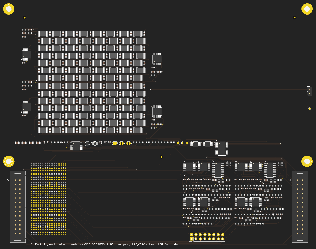
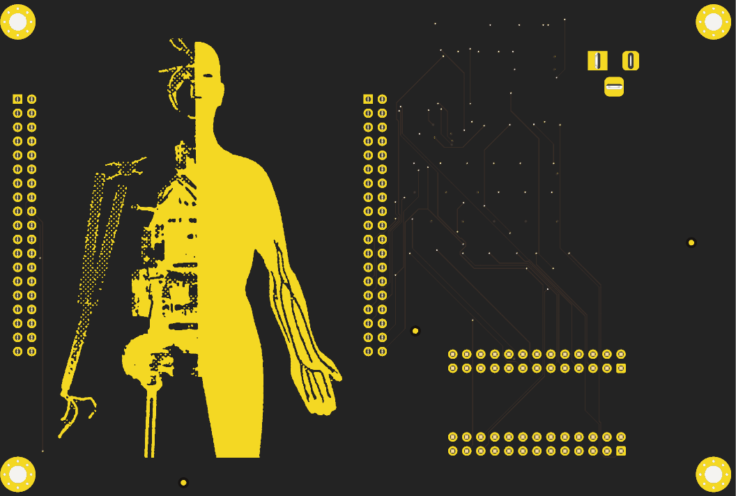
Board status
| Board | State | Checks |
|---|---|---|
| Carrier, with gold artwork | routed | 0 DRC violations |
| TILE-8 layer 1, 2 of 8 lines | routed | 0 DRC violations, 0 unrouted |
| TILE-8 layer 2, 8 lines | placed, not routed | 499 unconnected items |
| TILE-8 layer 3, 8 lines | placed, not routed | same as layer 2 |
Estimated bill of materials, three designs side by side
| Crosstalk, width 8 × 3 | 1-D CNN on the carrier’s microcontroller | Crosstalk, width 32 × 4 | |
|---|---|---|---|
| Parts | $191 (three tiles, carrier) | — | — |
| Circuit boards | $52 | — | — |
| Assembly | $129 | — | — |
| Microcontroller, cables, supply | $34 | $34 | $34 |
| Total, estimated | $406 · $507–549 with 25% contingency | $34 | ≈ $4,135 |
| Tiles | 3 | 0 | 52 |
| Inductors | 1,008 | 0 | 21,952 |
| Solder joints, tiles | 7,811 | — | — |
| Weights | 1,152 ternary, held as 716 fitted resistors | 1,248 parameters, float, in flash | ternary, held as resistors |
| Accuracy, simulated | 0.878 board line · 0.8705 parasitics tier | 0.909 | 0.931 virtual |
| Energy per classification | ≈ 162 µJ, design current | ≥ 84 µJ, lower bound | — |
| Changing the weights | a new assembly order | reflash, seconds | a new assembly order |
| State | designed, not built | not run on hardware here | simulated only |
A full tile costs about $75.89 in parts, $44.49 of it inductors. Five things still need checking before anyone orders one: the microcontroller header’s geometry, the assembler’s rotation offsets, how the inductors are oriented and coupled, a firm quote, and the 3.3 V bias network, which so far has passed only an automated electrical check.
Scaling up is expensive. Every input channel needs its own delay line, and each tile carries eight lines and eight outputs, so a layer of width W needs tiles. A network of depth D needs this many inductors: .
Scaling with network width
| Width × depth | Tiles | Inductors | Accuracy (V tier) |
|---|---|---|---|
| 8 × 3 (demonstrator) | 3 | 1,008 | 0.806 |
| 16 × 4 | 14 | 5,600 | — |
| 32 × 4 | 52 | 21,952 | 0.931 |
| 64 × 6 | 328 | 144,256 | — |
How tall a stack of tiles each model would need
- Established
- A ternary network whose weights are entries in a pick-and-place file, carried from training to a routed tile, with a design error found in simulation before any order was placed.
- Not established
- Any accuracy or energy advantage over conventional models at this size: the floating-point CNN and a 208-parameter classifier both do better.
- Open
- Running the C (circuit) tier end to end, routing the full tiles, and any measurement on hardware. Measuring twenty inductors on a Q meter would be a start.
Method and sources
Code: github.com/drksci/crosstalk (formerly delaytensor), packages/delay-tensor (configs tensor_8x64, tensor_16x128, mnist_8x784) and benches/, working tree of 4 November 2026 including uncommitted MNIST and RF work. Runs: seeds 1234, 1235, 1236; stratified 25% hold-out for the synthetic tasks, the canonical MNIST split for MNIST. Readout: StandardScaler and LogisticRegression (C = 1, lbfgs) for the synthetic tasks, the same model fitted by SGD for MNIST. Benches: ngspice 41 via PySpice, scikit-rf. Hardware: a 4-thread Intel laptop with 8 GB of memory. The experiments, tests and run data in both parts were produced by Claude Code sessions, mostly on the Fable model, under the author’s direction. The section 1 board drawing is a build123d model with hidden lines removed; it illustrates the idea. Part two was read from the project’s files and not re-run: its numbers come from the project’s data files, claim list (217 claims, checked by its own verify notebook) and article draft, at delaytensor main 15b30f4; its board images are KiCad renders. The C-tier result for the board network comes from the package’s circuit-extraction notes, which are newer than its draft; the E tier on the board network is still pending.
- classify · six-way synthetic waveforms, tensor_8x64, three seeds
- xor · temporal XOR, tensor_8x64, three seeds
- mnist · raw pixels, tensor features and MLP, mnist_8x784, three seeds
- Ablation sweeps · coupling, decay, readout, nonlinearity, mask mode, size; one knob per run, run for this piece
- Equivalence bench · update rule unrolled to 2,048 stages, ngspice operating point against NumPy
- RF bench · RLCG topologies, ngspice AC and transient, analytic chain matrix, scikit-rf referee, state-space extraction
- Design notes and tooling survey
- phase-lattice (dllm) · the original PyTorch prototype, five commits, one recorded result
- Crosstalk arena · nine models on 8-class synthetic modulation recognition, 16,000 / 4,000 windows
- Crosstalk P (parasitics) tier · parasitics model, gain-trim and crosstalk sweeps, 1,000-board Monte Carlo
- Crosstalk ladder tap response · ngspice .ac of the KiCad-exported tile, Q 10 and Q 30
- Crosstalk boards · KiCad 9 carrier and TILE-8 tiles, ERC/DRC reports, renders, BOM and cost model
- Crosstalk article draft and claim list · source of the prior-art survey and the energy references (Horowitz, ISSCC 2014; STM32G474 DS12288 Rev 2)
- Board drawing · build123d model, isometric projection, hidden lines removed
Delay lines began as radar equipment. Tubes of mercury held one sweep of echoes so that only moving targets showed on the screen, and the first stored-program computers borrowed the trick, keeping their working memory as sound circulating through mercury or coiled wire, readable only at one end.
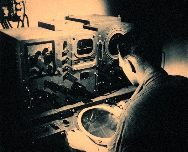
Radar technician at a radar display — Mercury delay lines were first built for wartime radar, to cancel echoes that had not moved.
Computer History Museum, catalogue 500004583 · © Computer History Museum
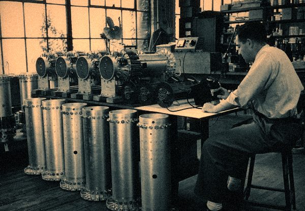
Technician with mercury delay lines — A technician checks mercury delay-line memory for the UNIVAC I.
Computer History Museum, catalogue 102722391 · © Computer History Museum
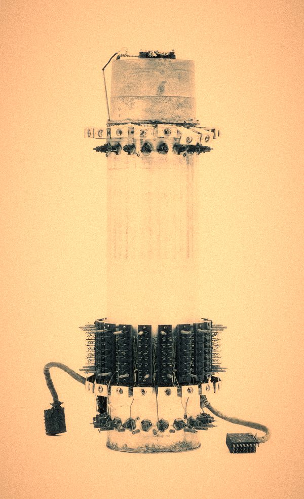
UNIVAC I delay-line memory, central support — A set of these gave the UNIVAC I about 1.5 KB of memory. Filled with mercury, each tank weighed nearly 800 lb.
Computer History Museum, catalogue 102677540 · © Computer History Museum
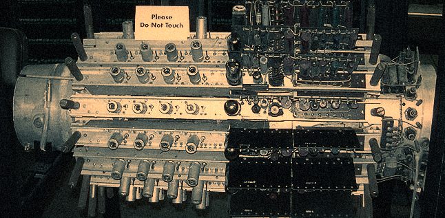
Mercury memory — Mercury delay-line memory of the kind used in the UNIVAC I.
Wikimedia Commons, File:Mercury_memory.jpg · CC BY-SA 3.0

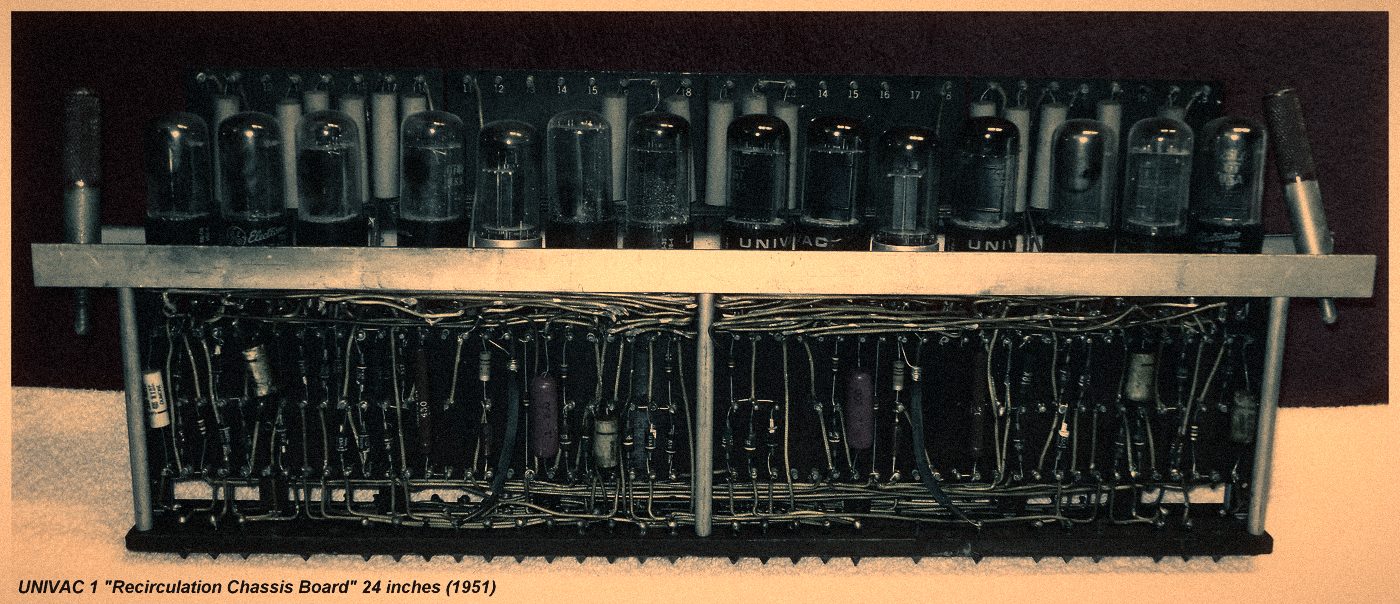
UNIVAC I recirculation chassis — The vacuum-tube board that re-amplified and re-timed the bits leaving a tank and sent them round again. 24 inches long.
Mark Greenia, Wikimedia Commons · CC BY-SA 4.0

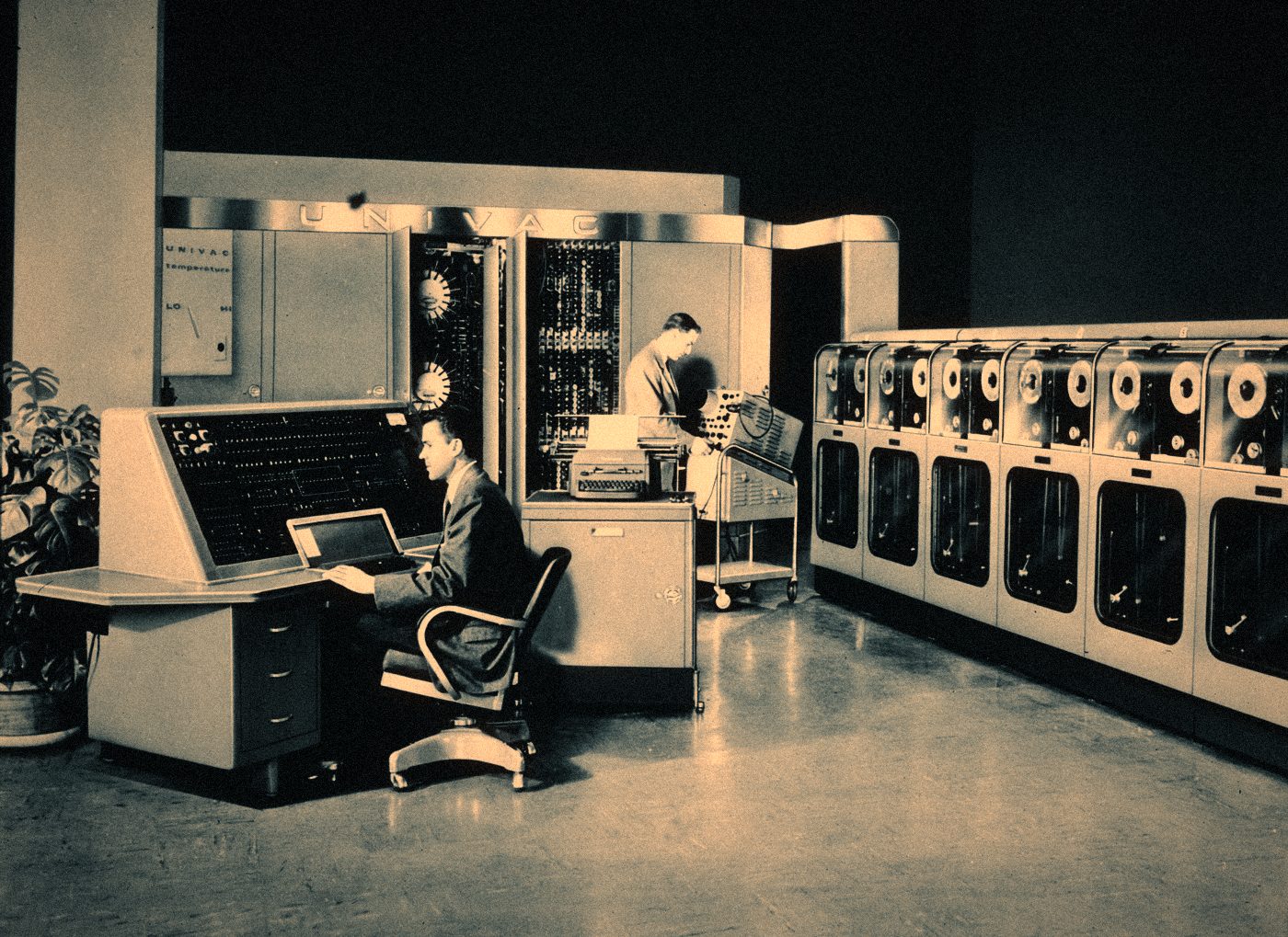
UNIVAC I dedication, US Census Bureau — The first UNIVAC I, dedicated at the Eckert-Mauchly plant in Philadelphia for the Census Bureau.
US Census Bureau, via Wikimedia Commons · Public domain

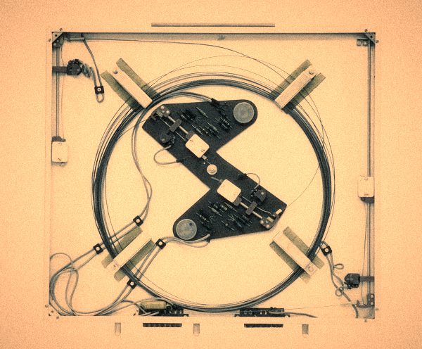
Ferranti Sirius magnetostrictive delay line — The same circulating memory without mercury: a strip of special metal rolled into a coil, with a transducer at each end.
Computer History Museum, catalogue XD230.80 · © Computer History Museum